A project is the most basic format in eCognition Architect. A project contains one or more maps and optionally a related rule set. Projects can be saved separately as a .dpr project file, but one or more projects can also be stored as part of a workspace.
For more advanced applications, workspaces reference the values of exported results and hold processing information such as import and export templates, the required ruleware, processing states, and the required software configuration. A workspace is saved as a set of files that are referenced by a .dpj file.
To create a simple project – one without metadata, or scaling (geocoding is detected automatically) – go to File > Load Image File in the main menu.
In Windows there is a 260-character limit on filenames and filepaths http://msdn.microsoft.com/en-us/library/windows/desktop/aa365247%28v=vs.85%29.aspx. Trimble software does not have this restriction and can export paths and create workspaces beyond this limitation. For examples of this feature, refer to the FAQs in the Windows installation guide.
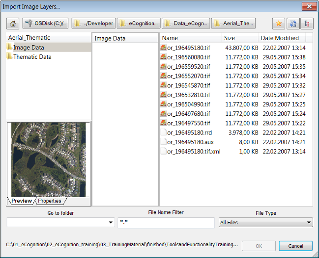
Load Image File (along with Open Project, Open Workspace and Load Ruleset) uses a customized dialog box. Selecting a drive displays sub-folders in the adjacent pane; the dialog will display the parent folder and the subfolder.
Clicking on a sub-folder then displays all the recognized file types within it (this is the default).
You can filter file names or file types using the File Name field. To combine different conditions, separate them with a semicolon (for example *.tif; *.las). The File Type drop-down list lets you select from a range of predefined file types.
The buttons at the top of the dialog box let you easily navigate between folders. Pressing the Home button returns you to the root file system.

There are three additional buttons available. The Add to Favorites button on the left lets you add a shortcut to the left-hand pane, which are listed under the Favorites heading. The second button, Restore Layouts, tidies up the display in the dialog box. The third, Search Subfolders, additionally displays the contents of any subfolders within a folder. You can, by holding down Ctrl or Shift, select more than one folder. Files can be sorted by name, size and by date modified.
In the Load Image File dialog box you can:
To later add additional image or thematic layers go to File > Add Data Layer in the main menu.
The Source View dialog provides users a simple data management area to modify input layer alias, display orders and access information on file details.
To open the dialog choose View > Source View.
 Select the Add input layer button to load data files, alternatively you can select the files in the Windows File Explorer and drag and drop them to the dialog to import them. You can add image layers, vector and point cloud layers to a new or existing project.
Furthermore, eCognition project (.dpr) and workspace (.dpj) files can be added by drag and drop.
 This button deletes a selected data layer or a whole project (dependent on selection).
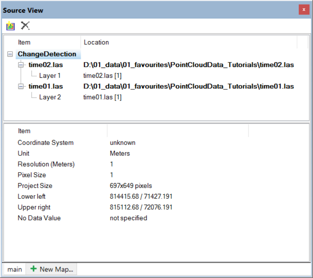
The upper pane of the Source View dialog shows the project name, all data layers loaded, their alias and file paths. On selection of a project file or data file the lower pane shows different details and settings.
If you right click in the upper pane on the project name or a data file you can select one of the following options from the context menu:
The lower pane of the Source View dialog shows the following details
A) on selection of a project:
B) on selection of a data file:
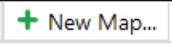 Use this dialog to add new maps to your project. Once you have added new maps, you can switch between their properties using the tabs at the bottom of the dialog.
When you create a new project, the software generates a main map representing the image data of a scene. To prepare this, you select image layers and optional data sources like thematic layers or metadata for loading to a new project. You can rearrange the image layers, select a subset of the image or modify the project default settings. In addition, you can add metadata.
An image file contains one or more image layers. For example, an RGB image file contains three image layers, which are displayed through the Red, Green and Blue channels (layers).
Open the Create Project dialog box by going to File > New Project (for more detailed information on creating a project, refer to The Create Project Dialog Box). The Import Image Layers dialog box opens. Select the image data you wish to import, then press the Open button to display the Create Project dialog box.
Opening certain file formats or structures requires you to select the correct driver in the File Type drop-down list.
Then select from the main file in the files area. If you select a repository file (archive file), another Import Image Layers dialog box opens, where you can select from the contained files. Press Open to display the Create Project dialog box.
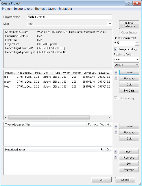
The Create Project dialog box gives you several options. These options can be edited at any time by selecting File > Modify Open Project:
In special cases you may want to ignore the unit information from the included geocoding information. To do so, deactivate Initialize Unit Conversion from Input File item in Tools > Options in the main menu
Geocoding is the assignment of positioning marks in images by coordinates. In earth sciences, position marks serve as geographic identifiers. But geocoding is helpful for life sciences image analysis too. Typical examples include working with subsets, at multiple magnifications, or with thematic layers for transferring image analysis results.
Typically, available geocoding information is automatically detected: if not, you can enter coordinates manually. Images without geocodes create automatically a virtual coordinate system with a value of 0/0 at the upper left and a unit of 1 pixel. For such images, geocoding represents the pixel coordinates instead of geographic coordinates.
The software cannot reproject image layers or thematic layers. Therefore all image layers must belong to the same coordinate system in order to be read properly. If the coordinate system is supported, geographic coordinates from inserted files are detected automatically. If the information is not included in the image file but is nevertheless available, you can edit it manually.
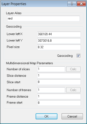
After importing a layer in the Create New Project or Modify Existing Project dialog boxes, double-click on a layer to open the Layer Properties dialog box. To edit geocoding information, select the Geocoding check box. You can edit the following:
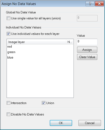
No-data values can be assigned to scenes with two dimensions only. This allows you to set the value of pixels that are not to be analyzed. Only no-data-value definitions can be applied to maps that have not yet been analyzed.
No-data values can be assigned to image pixel values (or combinations of values) to save processing time. These areas will not be included in the image analysis. Typical examples for no-data values are bright or dark background areas. The Assign No Data Value dialog box can be accessed when you create or modify a project.
After preloading image layers press the No Data button. The Assign No Data Values dialog box opens:
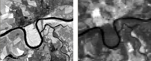
You can insert image layers and thematic layers with different resolutions (scales) into a map. They need not have the same number of columns and rows. To combine image layers of different resolutions (scales), the images with the lower resolution – having a larger pixel size – are resampled to the size of the smallest pixel size. If the layers have exactly the same size and geographical position, then geocoding is not necessary for the resampling of images.
When creating a new map, you can check and edit parameters of multidimensional maps that represent time series. Typically, these parameters are taken automatically from the image data set and this display is for checking only. However in special cases you may want to change the number, the distance and the starting item of frames. The preconditions for amending these values are:
To open the edit multidimensional map parameters, create a new project or add a map to an existing one. After preloading image layers press the Edit button. The Layer Properties dialog box opens.
Editable parameters are listed in the following table - Multidimensional Map Parameters:
| Parameter | Description | Calc button | Default |
|---|---|---|---|
| Number of frames | The number of two-dimensional images each representing a single film picture (frame) of a scene with time dimension. | Click the Calc button to calculate the rounded ratio of width and height of the internal map. | 1 |
| Frame distance | Change the temporal distance between frames. | (no influence) | 1 |
| Frame start | Change the number of the first displayed frame. | (no influence) | 0 |
Confirm with OK and return to the previous dialog box. After the a with a new map has been created or saved, the parameters of multidimensional maps cannot be changed any more.
If the loaded image files are geo-referenced to one single coordinate system, image layers and thematic layers with a different geographical coverage, size, or resolution can be inserted.
This means that image data and thematic data of various origins can be used simultaneously. The different information channels can be brought into a reasonable relationship to each other.
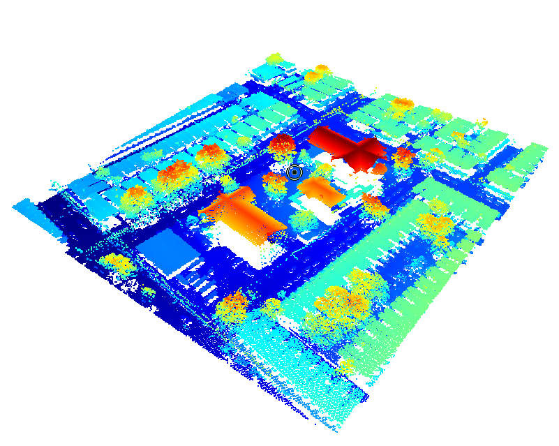
When dealing with Point Cloud processing and analysis, there are several components that provide you with the means to directly load and analyze point clouds, as well as to export result as raster images, such as DSM and DTM.
After loading, the point cloud is displayed in height rendering mode. To allow for quick display of the point cloud a rasterization is implemented in a simple averaging mode based on intensity values. This image layer can be activated in the View Settings dialog (with point cloud inactivated). Complex interpolation of the data can be done based on the Rasterize point cloud algorithm.
A) Select File > New Project
In the loading process, a resolution must be set that determines the grid spacing of the raster image generated from the las file. The resolution is set to 1 by default, which is the optimal value for point cloud data with a point density of 1pt/m2. For data with a lower resolution, set the value to 2 or above; for higher-resolution data, set it to 0.5 or below.
B) In the View Settings dialog
When working with point clouds, eCognition Developer uses the following approach:
 and draw a rectangle in the view (or alternatively select a non-parallel subset using View > Toolbars > 3D and select the 3 click 3D subset selection button to draw the rectangle).
Many image data formats include metadata or come with separate metadata files, which provide additional image information on content, qualitiy or condition of data. To use this metadata information in your image analysis, you can convert it into features and use these features for classification.
The available metadata depends on the data provider or camera used. Examples are:
The metadata provided can be displayed in the Image Object Information window, the Feature View window or the Select Displayed Features dialog box. For example depending on latitude and longitude a rule set for a specific vegetation zone can be applied to the image data.
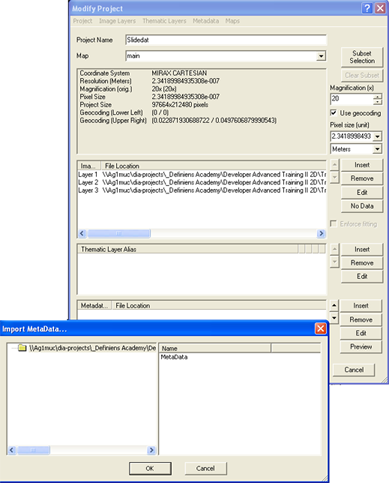
Although it is not usually necessary, you may sometimes need to link an open project to its associated metadata file. To add metadata to an open project, go to File > Modify Open Project.
The lowest pane of the Modify Project dialog box allows you to edit the links to metadata files. Select Insert to locate the metadata file. It is very important to select the correct file type when you open the metadata file to avoid error messages.
Once you have selected the file, select the correct field from the Import Metadata box and press OK. The filepath will then appear in the metadata pane.
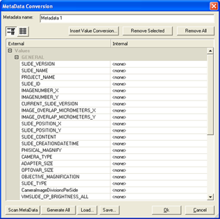
To populate with metadata, press the Edit button to launch the MetaData Conversion dialog box.
Press Generate All to populate the list with metadata, which will appear in the right-hand column. You can also load or save metadata in the form of XML files.
If you are batch importing large amounts of image data, then you should define metadata via the Customized Import dialog box.
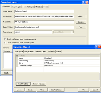
On the Metadata tab of the Customized Import dialog box, you can load Metadata into the projects to be created and thus modify the import template with regard to the following options:
A master file must be defined in the Workspace tab; if it is not, you cannot access the Metadata tab. The Metadata tab lists the metadata to be imported in groups and can be modified using the Add Metadata and Remove Metadata buttons.
You may want to use metadata in your analysis or in writing rule sets. Once the metadata conversion box has been generated, click Load – this will send the metadata values to the Feature View window, creating a new list under Metadata. Right-click on a feature and select Display in Image Object Information to view their values in the Image Object Information window.
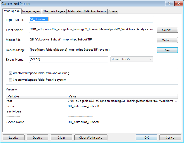
Multiple scenes from an existing file structure can be imported into a workspace and saved as an import template. The idea is that the user first defines a master file, which functions as a sample file and allows identification of the scenes of the workspace. The user then defines individual data that represents a scene by defining a search string.
A workspace must be in place before scenes can be imported and the file structure of image data to be imported must follow a consistent pattern. To open the Customized Import dialog box, go to the left-hand pane of the Workspace window and right-click a folder to select Customized Import. Alternatively select File > Customized Import from the main menu.
Add, move, and rename folders in the tree view on the left pane of the Workspace window. Depending on the import template, these folders may represent different items.
Workspaces are saved automatically whenever they are changed. If you create one or more copies of a workspace, changes to any of these will result in an update of all copies, irrespective of their location. Moving a workspace is easy because you can move the complete workspace folder and continue working with the workspace in the new location. If file connections related to the input data are lost, the Locate Image dialog box opens, where you can restore them; this automatically updates all other input data files that are stored under the same input root folder. If you have loaded input data from multiple input root folders, you only have to relocate one file per input root folder to update all file connections.
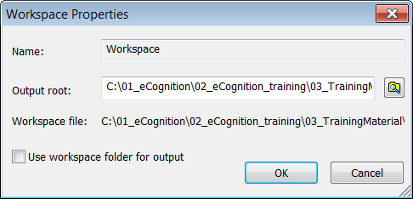
We recommend that you do not move any output files that are stored by default within the workspace folder. These are typically all .dpr project files and by default, all results files. However, if you do, you can modify the path of the output root folder under which all output files are stored.
To modify the path of the output root folder choose File > Workspace Properties from the main menu. Clear the Use Workspace Folder check-box and change the path of the output root folder by editing it, or click the Browse for Folders button and browse to an output root folder. This changes the location where image results and statistics will be stored. The workspace location is not changed.
Opening Projects and Workspace Subsets Open a project to view and investigate its maps in the map view:
For monitoring purposes you can view the state of the current version of a project. Go to the right-hand pane of the Workspace window that lists the projects. The state of a current version of a project is displayed behind its name.
| Processing States Related to User Workflow | |
|---|---|
| Created | Project has been created. |
| Canceled | Automated analysis has been canceled by the user. |
| Edited | Project has been modified automatically or manually. |
| Processed | Automated analysis has finished successfully. |
| Skipped | Tile was not selected randomly by the submit scenes for analysis algorithm with parameter Percent of Tiles to Submit defined smaller than 100. |
| Stitched | Stitching after processing has been successfully finished. |
| Accepted | Result has been marked by the user as accepted. |
| Rejected | Result has been marked by the user as rejected. |
| Deleted | Project was removed by the user. This state is visible in the Project History. |
| Other Processing States | |
| Unavailable | The Job Scheduler (a basic element of eCognition software) where the job was submitted is currently unavailable. It might have been disconnected or restarted. |
| Waiting | Project is waiting for automated analysis. |
| Processing | Automated analysis is running. |
| Failed | Automated analysis has failed. See Remarks column for details. |
| Timeout | Automated analysis could not be completed due to a timeout. |
| Crashed | Automated analysis has crashed and could not be completed. |
Inspecting older versions helps with testing and optimizing solutions. This is especially helpful when performing a complex analysis, where the user may need to locate and revert to an earlier version.
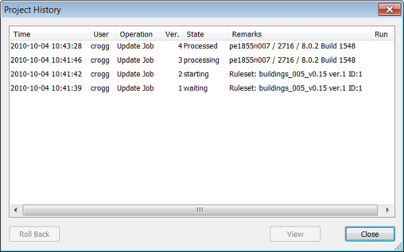
Clicking a column header lets you sort by column. To open a project version in the map view, select a project version and click View, or double-click a project version.
To restore an older version, choose the version you want to bring back and click the Roll Back button in the Project History dialog box. The restored project version does not replace the current version but adds it to the project version list. The intermediate versions are not lost.
Besides the Roll Back button in the Project History dialog box, you can manually revert to a previous version. (In the event of an unexpected processing failure, the project automatically rolls back to the last workflow state. This operation is documented as Automatic Rollback in the Remarks column of the Workspace window and as Roll Back Operation in the History dialog box.)
The intermediate versions are not lost. Select Destroy the History and All Results if you want to restart with a new version history after removing all intermediate versions including the results. In the Project History dialog box, the new version one displays Rollback in the Operations column.
Processed and unprocessed projects can be imported into a workspace.
Go to the left-hand pane of the Workspace window and select a folder. Right-click it and choose Import Existing Project from the context menu. Alternatively, Choose File > New Project from the main menu.
The Open Project dialog box will open. Select one project (file extension .dpr) and click Open; the new project is added to the right-hand Workspace pane.
To add multiple projects to a workspace, use the Import Scenes command. To add an existing projects to a workspace, use the Import Existing Project command. To create a new project separately from a workspace, close the workspace and use the Load Image File or New Project command.
Multi-map projects can be created from multiple scenes in a workspace. The preconditions to creating these are:
In the right-hand pane of the Workspace window select multiple projects by holding down the Ctrl or Shift key. Right-click and select Open from the context menu. Type a name for the new multi-map project in the opening New Multi-Map Project Name dialog box. Click OK to display the new project in the map view and add it to the project list.
If you select projects of different folders by using the List View, the new multi-map project is created in the folder with the last name in the alphabetical order. Example: If you select projects from a folder A and a folder B, the new multi-map project is created in folder B.
If you have to analyze projects with maps representing scenes that exceed the processing limitations, you have to consider some preparations.
Projects with maps representing scenes within the processing limitations can be processed normally, but some preparation is recommended if you want to accelerate the image analysis or if the system is running out of memory.
To handle such large scenes, you can work at different scales. If you process two-dimensional scenes, you have additional options:
For automated image analysis, we recommend developing rule sets that handle the above methods automatically. In the context of workspace automation, subroutines enable you to automate and accelerate the processing, especially the processing of large scenes.
When a project is removed, the related image data is not deleted. To remove one or more projects, select them in the right pane of the Workspace window. Either right-click the item and select Remove or press Del on the keyboard.
To remove folders along with their contained projects, right-click a folder in the left-hand pane of the Workspace window and choose Remove from the context menu.
If you removed a project by mistake, just close the workspace without saving. After reopening the workspace, the deleted projects are restored to the last saved version.
To save the currently displayed project list in the right-hand pane of the Workspace window to a .csv file:
In the Options dialog box under the Output Format group, you can define the decimal separator and the column delimiter according to your needs.
The current display of both panes of the Workspace can be copied the clipboard. It can then be pasted into a document or image editing program for example. Simply right-click in the right or left-hand pane of the Workspace Window and select Copy to Clipboard.
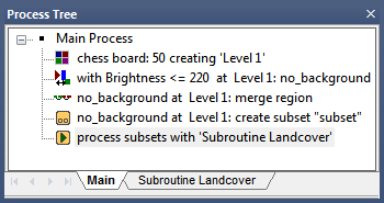
To give you practical illustrations of structuring a rule set into subroutines, have a look at some typical use cases including samples of rule set code. For detailed instructions, see the related instructional sections and the Reference Book listing all settings of algorithms.
Find regions of interest (ROIs), create scene subsets, and submit for further processing.
In this basic use case, you use a subroutine to limit detailed image analysis processing to subsets representing ROIs. The image analysis processes faster because you avoid detailed analysis of other areas.
Commonly, you use this subroutine use case at the beginning of a rule set and therefore it is part of the main process tree on the Main tab. Within the main process tree, you sequence processes in order to find regions of interest (ROI) on a bright background. Let us say that the intermediate results are multiple image objects of a class no_background representing the regions of interest of your image analysis task.
Still editing within the main process tree, you add a process applying the create scene subset algorithm on image objects of the class no_background in order to analyze regions of interest only.
The subsets created must be sent to a subroutine for analysis. Add a process with the algorithm submit scenes for analysis to the end of the main process tree. It executes a subroutine that defines the detailed image analysis processing on a separate tab.
Transfer intermediate result information by exporting to thematic layers and reloading them to a new scene copy. This subroutine use case presents an alternative for using the merging results parameters of the submit scenes for analysis algorithm because its intersection handling may result in performance intensive operations.
Here you use the export thematic raster files algorithm to export a geocoded thematic layer for each scene or subset containing classification information about intermediate results. This information, stored in a thematic layers and an associated attribute table, is a description of the location of image objects and information about the classification of image objects.
After exporting a geocoded thematic layer for each subset copy, you reload all thematic layers to a new copy of the complete scene. This copy is created using the create scene copy algorithm.
The subset thematic layers are matched correctly to the complete scene copy because they are geocoded. Consequently you have a copy of the complete scene with intermediate result information of preceding subroutines.
Using the submit scenes for analysis algorithm, you finally submit the copy of the complete scene for further processing to a subsequent subroutine. Here you can use the intermediate information of the thematic layer by using thematic attribute features or thematic layer operations algorithms.
Advanced: Transfer Results of Subsets
'at ROI_Level: export classification to ExportObjectsThematicLayer
'create scene copy 'MainSceneCopy'
'process 'MainSceneCopy*' subsets with 'Further'
Further
'Further Processing
''...
''...
''...
© 2019, Trimble Inc. All rights reserved. 