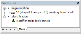
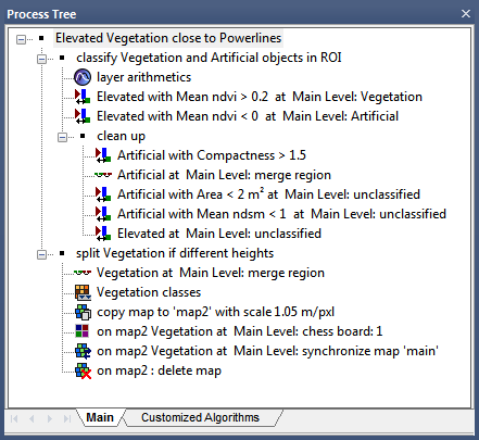
Rule sets are a combination of single processes, which are displayed in the Process Tree and created using the Edit Process dialog box. An existing rule set file (*.dcp) can be selected in the Windows File Explorer and imported by drag and drop into the Process Tree. A single process can operate on two levels; at the image object level (created by segmentation), or at the pixel level. Whatever the object, a process will run sequentially through each target, applying an algorithm to each. This section builds upon the tutorial in the previous chapter.
There are three ways to open the Edit Process dialog box:
To modify and see all parameters of a process the Process Properties window can be opened by selecting Process > Process Properties.
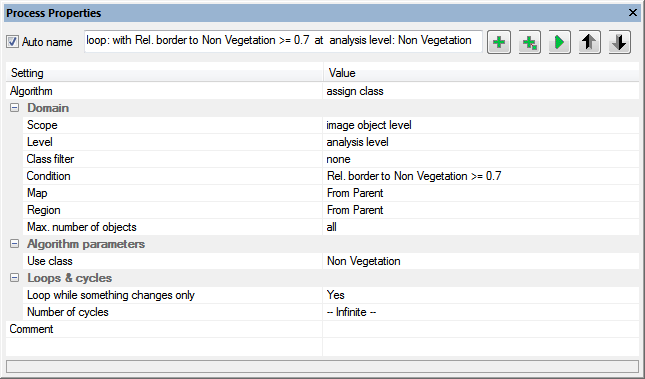
Use this dialog to append new processes, to insert child process and execute a selected process and navigate in your process tree up and down to visualize the respective processes.
Change the values of inserted algorithms by selecting the respective drop down menus in the value column.
When using the Process Properties window the domain section comprises the field Scope to select e.g. pixel level, image object level or vector domain.
The main functionality of the Process dialogs is explained in the following sections.
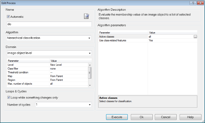
Naming of processes is automatic, unless the Automatic check-box is unchecked and a name is added manually. Processes can be grouped together and arranged into hierarchies, which has consequences around whether or not to use automatic naming – this is covered in Parent and Child Processes.
The Algorithm drop-down box allows the user to select an algorithm or a related process. Depending on the algorithm selected, further options may appear in the Algorithm Parameters pane.
This defines e.g. the image objects or vectors or image layers on which algorithms operate.
The domain parameters depend on the selected algorithm, details see Selecting and Configuring a Domain.
This defines the individual settings of the algorithm in the Algorithms Parameters group box. (We recommend you do this after selecting the domain.)
An algorithm can be applied to different areas or objects of interest – called domains in eCognition software. They allow to narrow down for instance the objects of interest and therefore the number of objects on which algorithms act.
For many algorithms the domain is defined by selecting a level within the image object hierarchy. Typical targets may be the pixel level, an image object level, or specified image objects but also single vector layers or a set of vector layers. When using the pixel level, the process creates a new image object level.
Depending on the algorithm, you can choose among different basic domains and specify your choice by setting execution parameters.
Main domain parameters are:
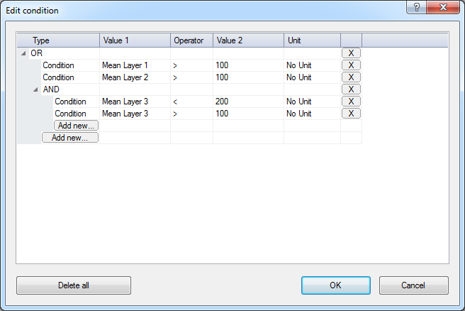
To define a condition enter a value, feature, or array item for both the value 1 and value 2 fields, and choose the desired operator.
Technically, the domain is a set of pixels, image objects, vectors or points. Every process loops through the set of e.g. image objects in the image object domain, one-by-one, and applies the algorithm to each image object.
The set of domains is extensible, using the eCognition Developer SDK. To specify the domain, select an image object level or another basic domain in the drop-down list. Available domains are listed in Domains.
| Basic Domain | Usage | Parameters |
|---|---|---|
| Execute | A general domain used to execute an algorithm. It will activate any commands you define in the Edit Process dialog box, but is independent of any image objects. It is commonly used to enable parent processes to run their subordinate processes (Execute Child Process) or to update a variable (Update Variable): Combined with threshold – if; Combined with map – on map; Threshold + Loop While Change – while | Condition; Map |
| Pixel level | Applies the algorithm to the pixel level. Typically used for initial segmentations and filters | Map; Condition |
| Image object level | Applies the algorithm to image objects on an image object level. Typically used for object processing | Level; Class filter; Condition; Map; Region; Max. number of objects |
| Current image object | Applies the algorithm to the current internally selected image object of the parent process. | Class filter; Condition; Max. number of objects |
| Neighbor image object | Applies the algorithm to all neighbors of the current internally selected image object of the parent process. The size of the neighborhood is defined by the Distance parameter. | Class filter; Condition; Max. number of objects; Distance |
| Super object | Applies the algorithm to the superobject of the current internally selected image object of the parent process. The number of levels up the image objects level hierarchy is defined by the Level Distance parameter. | Class filter; Condition; Level distance; Max. number of objects |
| Sub objects | Applies the algorithm to all sub-objects of the current internally selected image object of the parent process. The number of levels down the image objects level hierarchy is defined by the Level Distance parameter. | Class filter; Condition; Level distance; Max. number of objects |
| Linked objects | Applies the algorithm to the linked object of the current internally selected image object of the parent process. | Link class filter; Link direction; Max distance; Use current image object; Class filter; Condition; Max. number of objects |
| Maps | Applies the algorithm to all specified maps of a project. You can select this domain in parent processes with the Execute child process algorithm to set the context for child processes that use the Map parameter From Parent. | Map name prefix; Condition |
| Image object list | A selection of image objects created with the Update Image Object List algorithm. | Image object list; Class filter; Condition; Max. number of objects |
| Array | Applies the algorithm to a set of for example classes, levels, maps or multiple vector layers defined by an array. | Array; Array type; Index variable |
| Vectors | Applies the algorithm to a single vector layer. | Condition; Map; Thematic vector layer |
| Vectors (multiple layers) | Applies the algorithm to set of vector layers. | Condition; Map; Use Array; Thematic vector layers |
| Current vector | Applies the algorithm to the current internally selected vector object of the parent process. This domain is useful for iterating over individual vectors in a domain. | Condition |
This set of domains is extensible using the Developer SDK.

Algorithms are selected from the drop-down list under Algorithms; detailed descriptions of algorithms are available in the Reference Book.
By default, the drop-down list contains all available algorithms. You can customize this list by selecting ‘more’ from the drop-down list, which opens the Select Process Algorithms box.
By default, the ‘Display all Algorithms always’ box is selected. To customize the display, uncheck this box and press the left-facing arrow under ‘Move All’, which will clear the list. You can then select individual algorithms to move them to the Available Algorithms list, or double-click their headings to move whole groups.
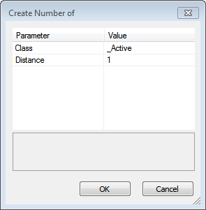
Loops & Cycles allows you to specify how many times you would like a process (and its child processes) to be repeated. The process runs cascading loops based on a number you define; the feature can also run loops while a feature changes (for example growing).
To execute a single process, select the process in the Process Tree and press F5. Alternatively, right-click on the process and select Execute. If you have child processes below your process, these will also be executed.
You can also execute a process from the Edit Process dialog box by pressing Execute, instead of OK (which adds the process to the Process Tree window without executing it).
To execute a process on an image object that as already been defined by a segmentation process, select the object then select the process in the Process Tree. To execute the process, right-click and select Execute on Selected Object or press F6.
The introductory tutorial introduces the concept of parent and child processes. Using this hierarchy allows you to organize your processes in a more logical way, grouping processes together to carry out a specific task.
Go to the Process Tree and right-click in the window. From the context menu, choose Append New. the Edit Process dialog will appear. This is the one time it is recommended that you deselect automatic naming and give the process a logical name, as you are essentially making a container for other processes. By default, the algorithm drop-down box displays Execute Child Processes. Press OK.
You can then add subordinate processes by right-clicking on your newly created parent and selecting Insert Child. We recommend you keep automatic naming for these processes, as the names display information about the process. Of course, you can select child process and add further child processes that are subordinate to these.
You can edit a process by double-clicking it or by right-clicking on it and selecting Edit; both options will display the Edit Process dialog box.
What is important to note is that when testing and modifying processes, you will often want to re-execute a single process that has already been executed. Before you can do this, however, you must delete the image object levels that these processes have created. In most cases, you have to delete all existing image object levels and execute the whole process sequence from the beginning. To delete image object levels, use the Delete Levels button on the main toolbar (or go to Image Objects > Delete Level(s) via the main menu).
It is also possible to delete a level as part of a rule set (and also to copy or rename one). In the Algorithm field in the Edit Process box, select Delete Image Object Level and enter your chosen parameters.
It is possible to go back to a previous state by using the undo function, which is located in Process > Undo (a Redo command is also available). These functions are also available as toolbar buttons using the Customize command. You can undo or redo the creation, modification or deletion of processes, classes, customized features and variables.
However, it is not possible to undo the execution of processes or any operations relating to image object levels, such as Copy Current Level or Delete Level. In addition, if items such as classes or variables that are referenced in rule sets are deleted and then undone, only the object itself is restored, not its references.
It is also possible to revert to a previous version.
You can assign a minimum number of undo actions by selecting Tools > Options; in addition, you can assign how much memory is allocated to the undo function (although the minimum number of undo actions has priority). To optimize memory you can also disable the undo function completely.
Right-clicking in the Process Tree window gives you two delete options:
Delete Rule Set eliminates all classes, variables, and customized features, in addition to all single processes. Consequently, an existing image object hierarchy with any classification is lost.
You can edit the organization of the Process Tree by dragging and dropping with the mouse. Bear in mind that a process can be connected to the Process Tree in three ways:
To drag and drop, go to the Process Tree window:
Commonly, the term segmentation means subdividing entities, such as objects, into smaller partitions. In eCognition Developer it is used differently; segmentation is any operation that creates new image objects or alters the morphology of existing image objects according to specific criteria. This means a segmentation can be a subdividing operation, a merging operation, or a reshaping operation.
There are two basic segmentation principles:
An analysis of which segmentation method to use with which type of image is beyond the scope of this guide; all the built-in segmentation algorithms have their pros and cons and a rule set developer must judge which methods are most appropriate for a particular image analysis.
Top-down segmentation means cutting objects into smaller objects. It can – but does not have to – originate from the entire image as one object. eCognition Developer offers three top-down segmentation methods: chessboard segmentation, quadtree-based segmentation and multi-threshold segmentation.
Multi-threshold segmentation is the most widely used; chessboard and quadtree-based segmentation are generally useful for tiling and dividing objects into equal regions.
Chessboard segmentation is the simplest segmentation algorithm. It cuts the scene or – in more complicated rule sets – the dedicated image objects into equal squares of a given size.
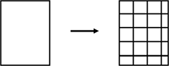
Because the Chessboard Segmentation algorithm produces simple square objects, it is often used to subdivide images and image objects. The following are some typical uses:
You can use the Edit Process dialog box to define the size of squares.
Quadtree-based segmentation is similar to chessboard segmentation, but creates squares of differing sizes. You can define an upper limit of color differences within each square using Scale Parameter. After cutting an initial square grid, the quadtree-based segmentation continues as follows:

Following a quadtree-based segmentation, very homogeneous regions typically produce larger squares than heterogeneous regions. Compared to multiresolution segmentation, quadtree-based segmentation is less heavy on resources.
Contrast filter segmentation is a very fast algorithm for initial segmentation and, in some cases, can isolate objects of interest in a single step. Because there is no need to initially create image object primitives smaller than the objects of interest, the number of image objects is lower than with some other approaches.
An integrated reshaping operation modifies the shape of image objects to help form coherent and compact image objects. The resulting pixel classification is stored in an internal thematic layer. Each pixel is classified as one of the following classes: no object, object in first layer, object in second layer, object in both layers and ignored by threshold. Finally, a chessboard segmentation is used to convert this thematic layer into an image object level.
In some cases you can use this algorithm as first step of your analysis to improve overall image analysis performance substantially. The algorithm is particularly suited to fluorescent images where image layer information is well separated.
Contrast split segmentation is similar to the multi-threshold segmentation approach. The contrast split segments the scene into dark and bright image objects based on a threshold value that maximizes the contrast between them.
The algorithm evaluates the optimal threshold separately for each image object in the domain. Initially, it executes a chessboard segmentation of variable scale and then performs the split on each square, in case the pixel level is selected in the domain.
Several basic parameters can be selected, the primary ones being the layer of interest and the classes you want to assign to dark and bright objects. Optimal thresholds for splitting and the contrast can be stored in scene variables.
Bottom-up segmentation means assembling objects to create a larger objects. It can – but does not have to – start with the pixels of the image. Examples are multiresolution segmentation and classification-based segmentation.
The Multiresolution Segmentation algorithm1 consecutively merges pixels or existing image objects. Essentially, the procedure identifies single image objects of one pixel in size and merges them with their neighbors, based on relative homogeneity criteria. This homogeneity criterion is a combination of spectral and shape criteria.
You can modify this calculation by modifying the scale parameter. Higher values for the scale parameter result in larger image objects, smaller values in smaller ones.
With any given average size of image objects, multiresolution segmentation yields good abstraction and shaping in any application area. However, it puts higher demands on the processor and memory, and is significantly slower than some other segmentation techniques – therefore it may not always be the best choice.
The homogeneity criterion of the multiresolution segmentation algorithm measures how homogeneous or heterogeneous an image object is within itself. It is calculated as a combination of the color and shape properties of the initial and resulting image objects of the intended merging.
Color homogeneity is based on the standard deviation of the spectral colors. The shape homogeneity is based on the deviation of a compact (or smooth) shape.2 Homogeneity criteria can be customized by weighting shape and compactness criteria:
The Multi-Threshold Segmentation algorithm splits the image object domain and classifies resulting image objects based on a defined pixel value threshold. This threshold can be user-defined or can be auto-adaptive when used in combination with the Automatic Threshold algorithm.
The threshold can be determined for an entire scene or for individual image objects; this determines whether it is stored in a scene variable or an object variable, dividing the selected set of pixels into two subsets so that heterogeneity is increased to a maximum. The algorithm uses a combination of histogram-based methods and the homogeneity measurement of multi-resolution segmentation to calculate a threshold dividing the selected set of pixels into two subsets.
Spectral difference segmentation lets you merge neighboring image objects if the difference between their layer mean intensities is below the value given by the maximum spectral difference. It is designed to refine existing segmentation results, by merging spectrally similar image objects produced by previous segmentations and therefore is a bottom-up segmentation.
The algorithm cannot be used to create new image object levels based on the pixel level.
All algorithms listed under the Reshaping Algorithms3 group technically belong to the segmentation strategies. Reshaping algorithms cannot be used to identify undefined image objects, because these algorithms require pre-existing image objects. However, they are useful for getting closer to regions and image objects of interest.
Sometimes reshaping algorithms are referred to as classification-based segmentation algorithms, because they commonly use information about the class of the image objects to be merged or cut. Although this is not always true, eCognition Developer uses this terminology.
The two most basic algorithms in this group are Merge Region and Grow Region. The more complex Image Object Fusion is a generalization of these two algorithms and offers additional options.
The Merge Region algorithm merges all neighboring image objects of a class into one large object. The class to be merged is specified in the domain.4

Classifications are not changed; only the number of image objects is reduced.
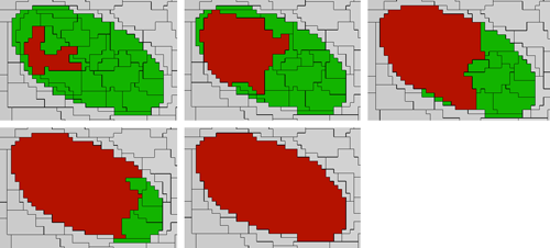
The Grow Region 5 algorithm extends all image objects that are specified in the domain, and thus represent the seed image objects. They are extended by neighboring image objects of defined candidate classes. For each process execution, only those candidate image objects that neighbor the seed image object before the process execution are merged into the seed objects. The following sequence illustrates four Grow Region processes:
Although you can perform some image analysis on a single image object level, the full power of the eCognition object-oriented image analysis unfolds when using multiple levels. On each of these levels, objects are defined by the objects on the level below them that are considered their sub-objects. In the same manner, the lowest level image objects are defined by the pixels of the image that belong to them. This concept has already been introduced in Image Object Hierarchy.
The levels of an image object hierarchy range from a fine resolution of image objects on the lowest level to the coarse resolution on the highest. On its superlevel, every image object has only one image object, the superobject. On the other hand, an image object may have – but is not required to have – multiple sub-objects.
To better understand the concept of the image object hierarchy, imagine a hierarchy of image object levels, each representing a meaningful structure in an image. These levels are related to the various (coarse, medium, fine) resolutions of the image objects. The hierarchy arranges subordinate image structures (such as a tree) below generic image structures (such as tree types); the figure below shows a geographical example.
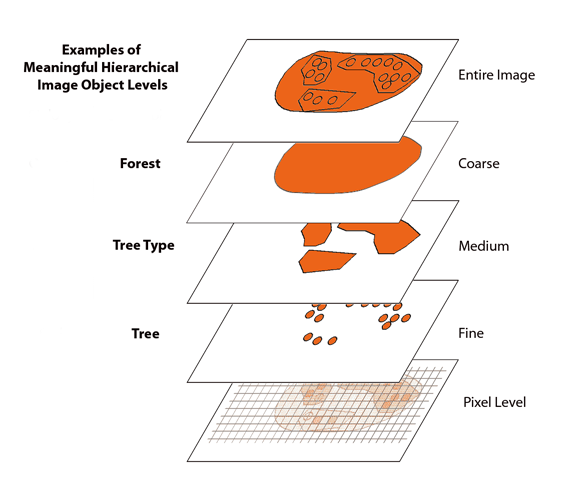
The lowest and highest members of the hierarchy are unchanging; at the bottom is the digital image itself, made up of pixels, while at the top is a level containing a single object (such as a forest).
There are two ways to create an image object level:
The shapes of image objects on these super- and sublevels will constrain the shape of the objects in the new level.
The hierarchical network of an image object hierarchy is topologically definite. In other words, the border of a superobject is consistent with the borders of its sub-objects. The area represented by a specific image object is defined by the sum of its sub-objects’ areas; eCognition technology accomplishes this quite easily, because the segmentation techniques use region-merging algorithms. For this reason, not all the algorithms used to analyze images allow a level to be created below an existing one.
Each image object level is constructed on the basis of its direct sub-objects. For example, the sub-objects of one level are merged into larger image objects on level above it. This merge is limited by the borders of exiting superobjects; adjacent image objects cannot be merged if they have different superobjects.
You can create an image object level by using some segmentation algorithms such as multiresolution segmentation, multi-threshold or spectral difference segmentation. The relevant settings are in the Edit Process dialog box:
Because a new level produced by segmentation uses the image objects of the level beneath it, the function has the following restrictions:
This structure enables you to create an image object hierarchy by segmenting the image multiple times, resulting in different image object levels with image objects of different scales.
It is often useful to duplicate an image object level in order to modify the copy. To duplicate a level, do one of the following:
You may want to rename an image object level name, for example to prepare a rule set for further processing steps or to follow your organization’s naming conventions. You can also create or edit level variables and assign them to existing levels.
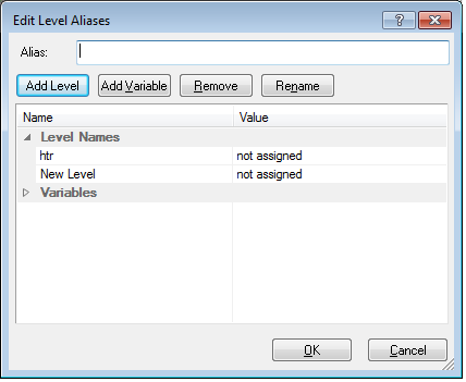
In some cases it is helpful to define names of image object levels before they are assigned to newly created image object levels during process execution. To do so, use the Add Level button within the Edit Level Aliases dialog box.
Instead of selecting any item in the drop-down list, just type the name of the image object level to be created during process execution. Click OK and the name is listed in the Edit Level Aliases dialog box.
When working with image object levels that are temporary, or are required for testing processes, you will want to delete image object levels that are no longer used. To delete an image object level do one of the following:
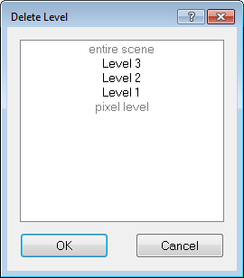
The Delete Level dialog box will open, which displays a list of all image object levels according to the image object hierarchy.
Select the image object level to be deleted (you can press Ctrl to select multiple levels) and press OK. The selected image object levels will be removed from the image object hierarchy. Advanced users may want to switch off the confirmation message before deletion. To do so, go to the Option dialog box and change the Ask Before Deleting Current Level setting.
The Image Object Information window is open by default, but can also be selected from the View menu if required. When analyzing individual images or developing rule sets you will need to investigate single image objects.
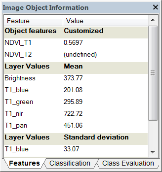
The Features tab of the Image Object Information window is used to get information on a selected image object.
Image objects consist of spectral, shape, and hierarchical elements. These elements are called features in eCognition Developer. The Feature tab in the Image Object Information window displays the values of selected attributes when an image object is selected in the view.
To get information on a specific image object click on an image object in the map view (some features are listed by default). To add or remove features, right-click the Image Object Information window and choose Select Features to Display. The Select Displayed Features dialog box opens, allowing you to select a feature of interest.
The selected feature values are now displayed in the view. To compare single image objects, click another image object in the map view and the displayed feature values are updated.
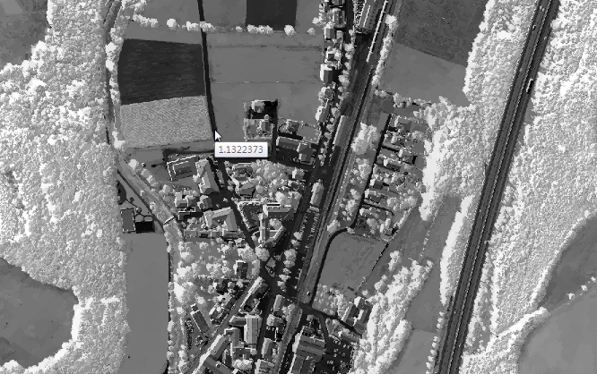
Double-click a feature to display it in the map view; to deselect a selected image object, click it in the map view a second time. If the processing for image object information takes too long, or if you want to cancel the processing for any reason, you can use the Cancel button in the status bar.
Image objects have spectral, shape, and hierarchical characteristics and these features are used as sources of information to define the inclusion-or-exclusion parameters used to classify image objects.
The major types of features are:
Available features are sorted in the feature tree, which is displayed in the Feature View window. It is open by default but can be also selected via Tools > Feature View or View > Feature View. A search field on top of the dialog allows quick navigation to any feature based on its name.

This section lists a very brief overview of functions. For more detailed information, consult the Reference Book.
Vector features are available in the feature tree if the project includes a thematic layer. They allow addressing vectors by their attributes, geometry and position features.
Object features are calculated by evaluating image objects themselves as well as their embedding in the image object hierarchy. They are grouped as follows:
Class features are dependent on image object features and refer to the classes assigned to image objects in the image object hierarchy.
This location is specified for superobjects and sub-objects by the levels separating them. For neighbor image objects, the location is specified by the spatial distance. Both these distances can be edited. Class features are grouped as follows:
Linked Object features are calculated by evaluating linked objects themselves.
Scene features return properties referring to the entire scene or map. They are global because they are not related to individual image objects, and are grouped as follows:
Process features are image object dependent features. They involve the relationship of a child process image object to a parent process. They are used in local processing.
A process features refers to a relation of an image objects to a parent process object (PPO) of a given process distance in the process hierarchy. Commonly used process features include:
Region features return properties referring to a given region. They are global because they are not related to individual image objects. They are grouped as follows:
Metadata items can be used as a feature in rule set development. To do so, you have to provide external metadata in the feature tree. If you are not using data import procedures to convert external source metadata to internal metadata definitions, you can create individual features from a single metadata item.
Feature variables have features as their values. Once a feature is assigned to a feature variable, the variable can be used in the same way, returning the same value and the assigned value. It is possible to create a feature variable without a feature assigned, but the calculation value would be invalid.
Most features with parameters must first be created before they are used and require values to be set beforehand. Before a feature of image object can be displayed in the map view, an image must be loaded and a segmentation must be applied to the map.
You can change the default feature unit for newly created features. Go to the Options dialog box and change the default feature unit item from pixels to ‘same as project unit’. The project unit is defined when creating the project and can be checked and modified in the Modify Project dialog box.
Thematic attributes can only be used if a thematic layer has been imported into the project. If this is the case, all thematic attributes in numeric form that are contained in the attribute table of the thematic layer can be used as features in the same manner as you would use any other feature.
Object-oriented texture analysis allows you to describe image objects by their texture. By looking at the structure of a given image object’s sub-objects, an object’s form and texture can be determined. An important aspect of this method is that the respective segmentation parameters of the sub-object level can easily be adapted to come up with sub-objects that represent the key structures of a texture.
A straightforward method is to use the predefined texture features provided by eCognition Developer. They enable you to characterize image objects by texture, determined by the spectral properties, contrasts and shape properties of their sub-objects.
Another approach to object-oriented texture analysis is to analyze the composition of classified sub objects. Class features (relations to sub objects) can be utilized to provide texture information about an image object, for example, the relative area covered by sub objects of a certain classification.
Further texture features are provided by Texture after Haralick7. These features are based upon the co-occurrence matrix, which is created out of the pixels of an object.
Some features may be edited to specify a distance relating two image objects. There are different types of feature distances:
The feature distance can be edited in the same way:
The level distance represents the hierarchical distance between image objects on different levels in the image object hierarchy. Starting from the current image object level, the level distance indicates the hierarchical distance of image object levels containing the respective image objects (sub-objects or superobjects).
The spatial distance represents the horizontal distance between image objects on the same level in the image object hierarchy.
Feature distance is used to analyze neighborhood relations between image objects on the same image object level in the image object hierarchy. It represents the spatial distance in the selected feature unit between the center of masses of image objects. The (default) value of 0 represents an exception, as it is not related to the distance between the center of masses of image objects; only the neighbors that have a mutual border are counted.
The process distance in the process hierarchy represents the upward distance of hierarchical levels in process tree between a process and the parent process. It is a basic parameter of process features.
In practice, the distance is the number of hierarchy levels in the Process Tree window above the current editing line, where you find the definition of the parent object. In the Process Tree, hierarchical levels are indicated using indentation.

To open this dialog select Image Objects > Image Object Table from the main menu.
This dialog allows you to compare image objects of selected classes when evaluating classifications. To launch the Configure Image Object Table dialog box, double-click in the window or right-click on the window and choose Configure Image Object Table.
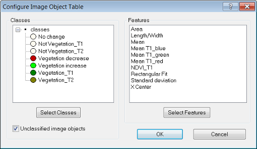
Upon opening, the classes and features windows are blank. Press the Select Classes button, which launches the Select Classes for List dialog box.
Add as many classes as you require by clicking on an individual class, or transferring the entire list with the All button. On the Configure Image Object Table dialog box, you can also add unclassified image objects by ticking the check box. In the same manner, you can add features by navigating via the Select Features button.
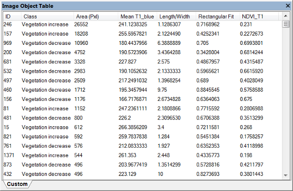
Clicking on a column header will sort rows according to column values. Depending on the export definition of the used analysis, there may be other tabs listing dedicated data. Selecting an object in the image or in the table will highlight the corresponding object.
In some cases an image analyst wants to assign specific annotations to single image objects manually, e.g. to mark objects to be reviewed by another operator. To add an annotation to an object right-click an item in the Image Object Table window and select Edit Object Annotation. The Edit Annotation dialog opens where you can insert a value for the selected object. Once you inserted the first annotation a new object variable is added to your project.
To display annotations in the Image Object Table window please select Configure Image Object Table again via right-click (see above) and add the Object feature > Variables > Annotation to the selected features.
Additionally, the feature Annotation can be found in the Feature View dialog > Object features > Variables > Annotation. Right-click this feature in the Feature View and select Display in Image Object Information to visualize the values in this dialog. Double-click the feature annotation in the Image Object Information dialog to open the Edit Annotation dialog where you can insert or edit its again.
This feature allows you to analyze the correlation of two features of selected image objects. If two features correlate highly, you may wish to deselect one of them from the Image Object Information or Feature View windows. As with the Feature View window, not only spectral information maybe displayed, but all available features.
The Correlation display shows the Pearson’s correlation coefficient between the values of the selected features and the selected image objects or classes.

Many image data formats include metadata or come with separate metadata files, which provide additional image information on content, qualitiy or condition of data. To use this metadata information in your image analysis, you can convert it into features and use these features for classification.
The available metadata depends on the data provider or camera used. Examples are:
The metadata provided can be displayed in the Image Object Information window, the Feature View window or the Select Displayed Features dialog box. For example depending on latitude and longitude a rule set for a specific vegetation zone can be applied to the image data.
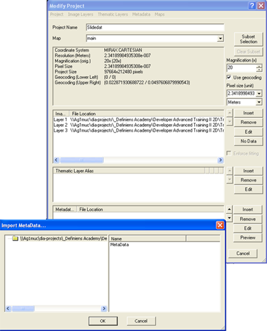
Although it is not usually necessary, you may sometimes need to link an open project to its associated metadata file. To add metadata to an open project, go to File > Modify Open Project.
The lowest pane of the Modify Project dialog box allows you to edit the links to metadata files. Select Insert to locate the metadata file. It is very important to select the correct file type when you open the metadata file to avoid error messages.
Once you have selected the file, select the correct field from the Import Metadata box and press OK. The filepath will then appear in the metadata pane.
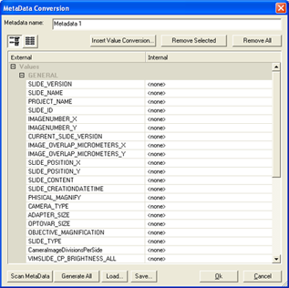
To populate with metadata, press the Edit button to launch the MetaData Conversion dialog box.
Press Generate All to populate the list with metadata, which will appear in the right-hand column. You can also load or save metadata in the form of XML files.
If you are batch importing large amounts of image data, then you should define metadata via the Customized Import dialog box.
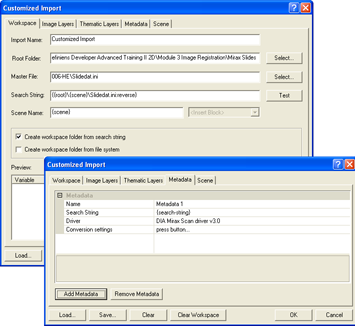
On the Metadata tab of the Customized Import dialog box, you can load Metadata into the projects to be created and thus modify the import template with regard to the following options:
A master file must be defined in the Workspace tab; if it is not, you cannot access the Metadata tab. The Metadata tab lists the metadata to be imported in groups and can be modified using the Add Metadata and Remove Metadata buttons.
You may want to use metadata in your analysis or in writing rule sets. Once the metadata conversion box has been generated, click Load – this will send the metadata values to the Feature View window, creating a new list under Metadata. Right-click on a feature and select Display in Image Object Information to view their values in the Image Object Information window.
1 Benz UC, Hofmann P, Willhauck G, Lingenfelder I (2004). Multi-Resolution, Object-Oriented Fuzzy Analysis of Remote Sensing Data for GIS-Ready Information. SPRS Journal of Photogrammetry & Remote Sensing, Vol 58, pp239–258. Amsterdam: Elsevier Science (↑)
2 The Multiresolution Segmentation algorithm criteria Smoothness and Compactness are not related to the features of the same name. (↑)
3 Sometimes reshaping algorithms are referred to as classification-based segmentation algorithms, because they commonly use information about the class of the image objects to be merged or cut. Although this is not always true, eCognition Developer uses this terminology. (↑)
4 The image object domain of a process using the Merge Region algorithm should define one class only. Otherwise, all objects will be merged irrespective of the class and the classification will be less predictable. (↑)
5 Grow region processes should begin the initial growth cycle with isolated seed image objects defined in the domain. Otherwise, if any candidate image objects border more than one seed image objects, ambiguity will result as to which seed image object each candidate image object will merge with. (↑)
6 You can change the default name for new image object levels in Tools > Options (↑)
7 The calculation of Haralick texture features can require considerable processor power, since for every pixel of an object, a 256 x 256 matrix has to be calculated. (↑)
© 2019, Trimble Inc. All rights reserved. 