A project is the most basic format in eCognition Developer. A project contains one or more maps and optionally a related rule set. Projects can be saved separately as a .dpr project file, but one or more projects can also be stored as part of a workspace.
For more advanced applications, workspaces reference the values of exported results and hold processing information such as import and export templates, the required ruleware, processing states, and the required software configuration. A workspace is saved as a set of files that are referenced by a .dpj file.
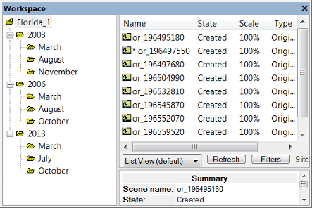
The Workspace window lets you view and manage all the projects in your workspace, along with other relevant data. You can open it by selecting View > Windows > Workspace from the main menu.
The Workspace window is split in two panes:
In List View and Folder View, information is displayed about a selected project – its state, scale, the time of the last processing and any available comments. The Scale column displays the scale of the scene. Depending on the processed analysis, there are additional columns providing exported result values.
To create a new workspace, select File > New Workspace from the main menu or use the Create New Workspace button on the default toolbar. The Create New Workspace dialog box lets you name your workspace and define its file location – it will then be displayed as the root folder in the Workspace window.
If you need to define another output root folder, it is preferable to do so before you load scenes into the workspace. However, you can modify the path of the output root folder later on using File > Workspace Properties.
Before you can start working on data, you must import scenes in order to add image data to the workspace. During import, a project is created for each scene. You can select different predefined import templates according to the image acquisition facility producing your image data.
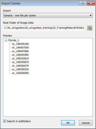
If you only want to import a single scene into a workspace, use the Add Project command. To import scenes to a workspace, choose File > Predefined Import from the main menu or right-click the left-hand pane of the Workspace window and choose Predefined Import. The Import Scenes dialog box opens.
Selecting Folder View gives you the option to display project statistics. Right-click in the right-hand pane and Select Folder Statistics Type from the drop-down menu. The available options are Sum, Mean, Standard Deviation, Minimum and Maximum.
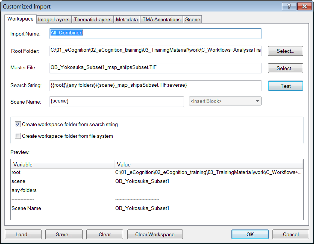
Multiple scenes from an existing file structure can be imported into a workspace and saved as an import template. The idea is that the user first defines a master file, which functions as a sample file and allows identification of the scenes of the workspace. The user then defines individual data that represents a scene by defining a search string.
A workspace must be in place before scenes can be imported and the file structure of image data to be imported must follow a consistent pattern. To open the Customized Import dialog box, go to the left-hand pane of the Workspace window and right-click a folder to select Customized Import. Alternatively select File > Customized Import from the main menu.
Press Save to save a template as an XML file. Templates are saved in custom folders that do not get deleted if eCognition Developer is uninstalled. Selecting Load will open the same folder – in Windows XP the location of this folder is C:\Documents and Settings\[User]\Application Data\eCognition\[Version Number]\Import. In Windows 7 and Windows 8 the location of this folder is C:\Users\[User]\AppData\Roaming\eCognition\[Version Number]\import.
Editing the Search String and the Scene Name – if the automatically generated ones are unsatisfactory – is often a challenge for less-experienced users.
There are two types of fields that you can use in search strings: static and variable. A static field is inserted as plain text and refers to file names or folder names (or parts of them). Variable fields are always enclosed in curly brackets and may refer to variables such as a layer, folder or scene. Variable fields can also be inserted from the Insert Block drop-down box.
For example, the expression {scene}001.tif will search for any scene whose filename ends in 001.tif. The expression {scene}_x_{scene}.jpg will find any JPEG file with _x_ in the filename.
For advanced editing, you can use regular expressions symbols such as:
"." (any single character),
"* " (zero or one of the preceding character),
".*" (by combining the dot and the star symbols you create a "wildcard"),
"|" (or operator), etc.
(Reference: https://autohotkey.com/docs/misc/RegEx-QuickRef.htm (visited 2016-04-15))
Here some examples for expressions:
{{root}\{any-folders}\{scene:"(A.*)"}.tif:reverse}
- creates scenes for *. tif images starting with "A" - Example: A_myimage.tif |
{{root}\{any-folders}\{scene:"(A.B)"}.tif:reverse}
- creates scenes for any *.tif image starting with "A", ending with "B", and with only one character in between - Example: a1b.tif, a2b.tif |
{{root}\{any-folders}\{scene:"((A|B).*)"}.tif:reverse}
- creates scenes for tif images with the character "A" or "B" at the beginning of the file name - Example: A_myimage.tif, B_myimage.tif) |
{{root}\{any-folders}\{scene:"(.*[0-9])"}.tif:reverse}
- create scenes for *.tif images with a digit at the end of the file name - Example: myimage1.tif, myimage2.tif |
{{root}\{any-folders}\{scene:"(.*\D)"}.tif:reverse}
- creates scenes for the tif images with a non-digit at the end of the file name - Example: my1_image.tif, my2_image.tif |
You must comply with the following search string editing rules:
| Block | Description | Usage |
|---|---|---|
| :reverse | Starts reading from the end instead of the beginning | {part of a file name:reverse} is recommended for reading file names, because file name endings are usually fixed |
| any | Represents any order and number of characters | Used as wildcard character for example, {any}.tif for TIFF files with an arbitrary name |
| any-folders | Represents one or multiples of nested folders down the hierarchy under which the image files are stored | {root}\ {any-folders}\ {any}.tif for all TIFF files in all folders below the root folder |
| root | Represents a root folder under which all image data you want to import is stored | Every search string has to start with {root}\ |
| folder | Represents one folder under which the image files are stored | {root}\{scene}.tif for TIFF files whose file names will be used as scene names |
| scene | Represents the name of a scene that will be used for project naming within the workspace after import | {root}\{scene}.tif for TIFF files whose file names will be used as scene names |
| layer | Represents the name of an image layer | |
| frame | Represents the frames of a time series data set. It can be used for files or folders. | {frame}.tif for all TIFF files or {frame}\{any}.tif for all TIFF files in a folder containing frame files. |
| column | Same as frame | Same as frame |
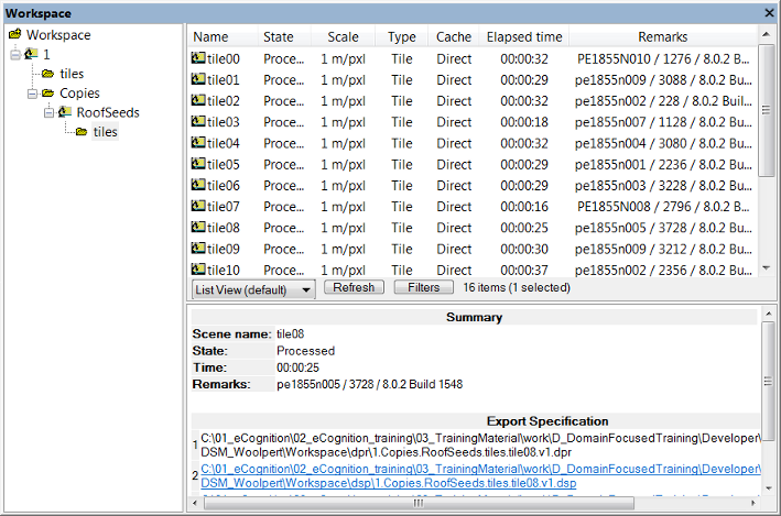
Projects in workspaces have compound names that include the path to the image data. Each folder2 within the Workspace window folder is part of the name that displays in the right-hand pane, with the name of the scene or tile included at the end. You can understand the naming convention by opening each folder in the left-hand pane of the Workspace window; the Scene name displays in the Summary pane. The name will also indicate any of the following:
Add, move, and rename folders in the tree view on the left pane of the Workspace window. Depending on the import template, these folders may represent different items.
Workspaces are saved automatically whenever they are changed. If you create one or more copies of a workspace, changes to any of these will result in an update of all copies, irrespective of their location. Moving a workspace is easy because you can move the complete workspace folder and continue working with the workspace in the new location. If file connections related to the input data are lost, the Locate Image dialog box opens, where you can restore them; this automatically updates all other input data files that are stored under the same input root folder. If you have loaded input data from multiple input root folders, you only have to relocate one file per input root folder to update all file connections.
We recommend that you do not move any output files that are stored by default within the workspace folder. These are typically all .dpr project files and by default, all results files. However, if you do, you can modify the path of the output root folder under which all output files are stored.
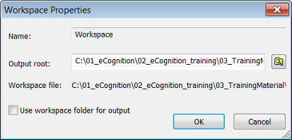
To modify the path of the output root folder choose File > Workspace Properties from the main menu. Clear the Use Workspace Folder check-box and change the path of the output root folder by editing it, or click the Browse for Folders button and browse to an output root folder. This changes the location where image results and statistics will be stored. The workspace location is not changed.
Opening Projects and Workspace Subsets Open a project to view and investigate its maps in the map view:
For monitoring purposes you can view the state of the current version of a project. Go to the right-hand pane of the Workspace window that lists the projects. The state of a current version of a project is displayed behind its name.
| Processing States Related to User Workflow | |
|---|---|
| Created | Project has been created. |
| Canceled | Automated analysis has been canceled by the user. |
| Edited | Project has been modified automatically or manually. |
| Processed | Automated analysis has finished successfully. |
| Skipped | Tile was not selected randomly by the submit scenes for analysis algorithm with parameter Percent of Tiles to Submit defined smaller than 100. |
| Stitched | Stitching after processing has been successfully finished. |
| Accepted | Result has been marked by the user as accepted. |
| Rejected | Result has been marked by the user as rejected. |
| Deleted | Project was removed by the user. This state is visible in the Project History. |
| Other Processing States | |
| Unavailable | The Job Scheduler (a basic element of eCognition software) where the job was submitted is currently unavailable. It might have been disconnected or restarted. |
| Waiting | Project is waiting for automated analysis. |
| Processing | Automated analysis is running. |
| Failed | Automated analysis has failed. See Remarks column for details. |
| Timeout | Automated analysis could not be completed due to a timeout. |
| Crashed | Automated analysis has crashed and could not be completed. |
Inspecting older versions helps with testing and optimizing solutions. This is especially helpful when performing a complex analysis, where the user may need to locate and revert to an earlier version.
Clicking a column header lets you sort by column. To open a project version in the map view, select a project version and click View, or double-click a project version.
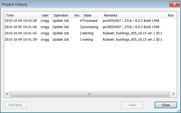
To restore an older version, choose the version you want to bring back and click the Roll Back button in the Project History dialog box. The restored project version does not replace the current version but adds it to the project version list. The intermediate versions are not lost.
Besides the Roll Back button in the Project History dialog box, you can manually revert to a previous version. (In the event of an unexpected processing failure, the project automatically rolls back to the last workflow state. This operation is documented as Automatic Rollback in the Remarks column of the Workspace window and as Roll Back Operation in the History dialog box.)
The intermediate versions are not lost. Select Destroy the History and All Results if you want to restart with a new version history after removing all intermediate versions including the results. In the Project History dialog box, the new version one displays Rollback in the Operations column.
Processed and unprocessed projects can be imported into a workspace.
Go to the left-hand pane of the Workspace window and select a folder. Right-click it and choose Import Existing Project from the context menu. Alternatively, Choose File > New Project from the main menu.
The Open Project dialog box will open. Select one project (file extension .dpr) and click Open; the new project is added to the right-hand Workspace pane.
To add multiple projects to a workspace, use the Import Scenes command. To add an existing projects to a workspace, use the Import Existing Project command. To create a new project separately from a workspace, close the workspace and use the Load Image File or New Project command.
Multi-map projects can be created from multiple scenes in a workspace. The preconditions to creating these are:
In the right-hand pane of the Workspace window select multiple projects by holding down the Ctrl or Shift key. Right-click and select Open from the context menu. Type a name for the new multi-map project in the opening New Multi-Map Project Name dialog box. Click OK to display the new project in the map view and add it to the project list.
If you select projects of different folders by using the List View, the new multi-map project is created in the folder with the last name in the alphabetical order. Example: If you select projects from a folder A and a folder B, the new multi-map project is created in folder B.
If you have to analyze projects with maps representing scenes that exceed the processing limitations, you have to consider some preparations.
Projects with maps representing scenes within the processing limitations can be processed normally, but some preparation is recommended if you want to accelerate the image analysis or if the system is running out of memory.
To handle such large scenes, you can work at different scales. If you process two-dimensional scenes, you have additional options:
For automated image analysis, we recommend developing rule sets that handle the above methods automatically. In the context of workspace automation, subroutines enable you to automate and accelerate the processing, especially the processing of large scenes.
When a project is removed, the related image data is not deleted. To remove one or more projects, select them in the right pane of the Workspace window. Either right-click the item and select Remove or press Del on the keyboard.
To remove folders along with their contained projects, right-click a folder in the left-hand pane of the Workspace window and choose Remove from the context menu.
If you removed a project by mistake, just close the workspace without saving. After reopening the workspace, the deleted projects are restored to the last saved version.
To save the currently displayed project list in the right-hand pane of the Workspace window to a .csv file:
In the Options dialog box under the Output Format group, you can define the decimal separator and the column delimiter according to your needs.
The current display of both panes of the Workspace can be copied the clipboard. It can then be pasted into a document or image editing program for example.
Simply right-click in the right or left-hand pane of the Workspace Window and select Copy to Clipboard.
Subscenes can be tiles or subsets. You can export statistics from a subscene analysis for each scene and collect and merge the statistical results of multiple files. The advantage is that you do not need to stitch the subscenes results for result operations concerning the main scene.
To do this, each subscene analysis must have had at least one project or domain statistic exported. All preceding subscene analysis, including export, must have been processed completely before the Read Subscene Statistics algorithm starts any result summary calculations. To ensure this, result calculations are done within a separate subroutine.
After processing all subscenes, the algorithm reads the exported result statistics of the subscenes and performs a defined mathematical summary operation. The resulting value, representing the statistical results of the main scene, is stored as a variable. This variable can be used for further calculations or export operations concerning the main scene.
A rule set with subroutines can be executed only on data loaded to a workspace. This enables you to review all projects of scenes, subset, and tiles. They all are stored in the workspace.
(A rule set with subroutines can only be executed if you are connected to an eCognition Server. Rule sets that include subroutines cannot be processed on a local machine.)
To give you practical illustrations of structuring a rule set into subroutines, have a look at some typical use cases including samples of rule set code. For detailed instructions, see the related instructional sections and the Reference Book listing all settings of algorithms.
Find regions of interest (ROIs), create scene subsets, and submit for further processing.
In this basic use case, you use a subroutine to limit detailed image analysis processing to subsets representing ROIs. The image analysis processes faster because you avoid detailed analysis of other areas.
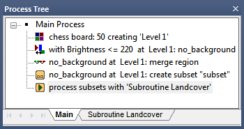
Commonly, you use this subroutine use case at the beginning of a rule set and therefore it is part of the main process tree on the Main tab. Within the main process tree, you sequence processes in order to find regions of interest (ROI) on a bright background. Let us say that the intermediate results are multiple image objects of a class no_background representing the regions of interest of your image analysis task.
Still editing within the main process tree, you add a process applying the create scene subset algorithm on image objects of the class no_background in order to analyze regions of interest only.
The subsets created must be sent to a subroutine for analysis. Add a process with the algorithm submit scenes for analysis to the end of the main process tree. It executes a subroutine that defines the detailed image analysis processing on a separate tab.
Transfer intermediate result information by exporting to thematic layers and reloading them to a new scene copy. This subroutine use case presents an alternative for using the merging results parameters of the submit scenes for analysis algorithm because its intersection handling may result in performance intensive operations.
Here you use the export thematic raster files algorithm to export a geocoded thematic layer for each scene or subset containing classification information about intermediate results. This information, stored in a thematic layers and an associated attribute table, is a description of the location of image objects and information about the classification of image objects.
After exporting a geocoded thematic layer for each subset copy, you reload all thematic layers to a new copy of the complete scene. This copy is created using the create scene copy algorithm.
The subset thematic layers are matched correctly to the complete scene copy because they are geocoded. Consequently you have a copy of the complete scene with intermediate result information of preceding subroutines.
Using the submit scenes for analysis algorithm, you finally submit the copy of the complete scene for further processing to a subsequent subroutine. Here you can use the intermediate information of the thematic layer by using thematic attribute features or thematic layer operations algorithms.
Advanced: Transfer Results of Subsets
'at ROI_Level: export classification to ExportObjectsThematicLayer
'create scene copy 'MainSceneCopy'
'process 'MainSceneCopy*' subsets with 'Further'
Further
'Further Processing
''...
''...
''...
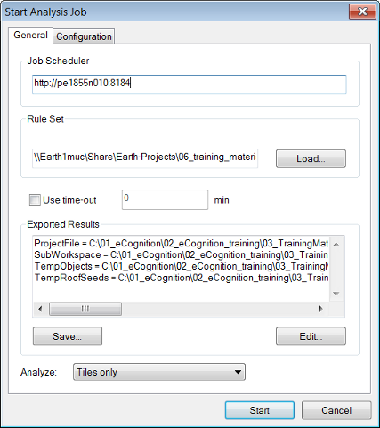
eCognition Developer enables you to perform automated image analysis jobs that apply rule sets to single or multiple projects. It requires a rule set or existing ruleware file, which may be a rule set (.dcp) or a solution (.dax). Select one or more items in the Workspace window – you can select one or more projects from the right-hand pane or an entire folder from the left-hand pane. Choose Analysis > Analyze from the main menu or right-click the selected item and choose Analyze. The Start Analysis Job dialog box opens.
If you want to repeat an automated image analysis, for example when testing, you need to rollback all changes of the analyzed projects to restore the original version. To determine which projects have been analyzed, go to the Workspace window and sort the State column. Select the Processed ones for rollback
These settings are designed for advanced users. Do not alter them unless you are aware of a specific need to change the default values and you understand the effects of the changes.
The Configuration tab of the Start Analysis Job dialog box enables you to review and alter the configuration information of a job before it is sent to the server. The configuration information for a job describes the required software and licenses needed to process the job. This information is used by the eCognition Server to configure the analysis engine software according to the job requirements.
An error message is generated if the installed packages do not meet the requirements specified in the Configuration tab. The configuration information is of three types: product, version and configuration.
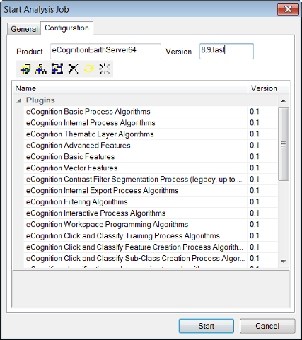
The Product field specifies the software package name that will be used to process the job. Packages are found by using pattern matching, so the default value ‘eCognition’ will match any package that begins with ‘eCognition’ and any such package will be valid for the job.
The Version field displays the default version of the software package used to process the job. You do not normally need to change the default.
If you do need to alter the version of the Analysis Engine Software, enter the number needed in the Version text box. If the version is available it will be used. The format for version numbers is major.upgrade.update.build. For example, 9.5.1.2543 means platform version 9.5.1, build 2543. You can simply use 9.5.last to use the latest installed software package with version 9.5.
The large pane at the bottom of the dialog box displays the plug-ins, data I/O drivers and extensions required by the analysis engine to process the job. The eCognition Grid will not start a software package that does not contain all the specified components.
The plug-ins that display initially are associated with the rule set that has been loaded in the General tab. All the listed plug-ins must be present for eCognition Server to process the rule set. You can also edit the plug-ins using the buttons at the top of the window.
To add a plug-in, first load a rule set on the General tab to display the associated plug-ins. Load a plug-in by clicking the Add Plug-in button or using the context menu to open the Add a Plug-In dialog box. Use the Name drop-down box to select a plug-in and version, if needed. Click OK to display the plug-in in the list.
The listed drivers listed must be installed for the eCognition Server to process the rule set. You might need to add a driver if it is required by the rule set and the wrong configuration is picked because of the missing information.
To add a driver, first load a rule set on the General tab to display the associated drivers. Load a driver by clicking the Add Driver button or using the context menu to open the Add a Driver dialog box. Use the drop-down Name list box to select a driver and optionally a version, if needed. Click OK to display the driver in the list.
You can also edit the version number in the list. For automatic selection of the correct version of the selected driver, delete the version number.
The Extension field displays extensions and applications, if available. To add an extension, first load a rule set on the General tab.
Load an extension by clicking the Add Extension button or using the context menu to open the Add an Extension dialog box. Enter the name of the extension in the Name field. Click OK to display the extension in the list.
To delete an item from the list, select the item and click the Delete Item button, or use the context menu. You cannot delete an extension.
If you have altered the initial configuration, return to the initial state by using the context menu or clicking the Reset Configuration Info button.
In the initial state, the plug-ins displayed are those associated with the rule set that has been loaded. Click the Load Client Config Info button or use the context menu to load the plug-in configuration of the client. For example, if you are using a rule set developed with an earlier version of the client, you can use this button to display all plug-ins associated with the client you are currently using.
Tiling and stitching is an eCognition method for handling large images. When images are so large that they begin to degrade performance, we recommend that they are cut into smaller pieces, which are then treated inpidually. Afterwards, the tile results are stitched together. The absolute size limit for an image in eCognition Developer is 231 (46,340 x 46,340 pixels).
Creating tiles splits a scene into multiple tiles of the same size and each is represented as a new map in a new project of the workspace. Projects are analyzed separately and the results stitched together (although we recommend a post-processing step).
Creating tiles is only suitable for 2D images. The tiles you create do not include results such as image objects, classes or variables.
To create a tile, you need to be in the Workspace window, which is displayed by default in views 1 and 3 on the main toolbar, or can be launched using View > Windows > Workspace. You can select a single project to tile its scenes or select a folder with projects within it.
To open the Create Tiles dialog box, choose Analysis > Create Tiles or select it by right-clicking in the Workspace window. The Create Tiles box allows you to enter the horizontal and vertical size of the tiles, based on the display unit of the project. For each scene to be tiled, a new tiles folder will be created, containing the created tile projects named tilenumber.
You can analyze tile projects in the same way as regular projects by selecting single or multiple tiles or folders that contain tiles.
Only the main map of a tile project can be stitched together. In the Workspace window, select a project with a scene from which you created tiles. These tiles must have already been analyzed and be in the ‘processed’ state. To open the Stitch Tile Results dialog box, select Analysis > Stitch Projects from the main menu or right-click in the Workspace window.
The Job Scheduler field lets you specify the computer that is performing the analysis. It is set to http://localhost:8184 by default, which is the local machine. However, if you are running eCognition Developer over a network, you may need change this field to the address of another computer.
Click Load to load a ruleware file for image analysis — this can be a process (.dcp) or solution (.dax) file. The Edit feature allows you to configure the exported results and the export paths of the image analysis job in an export template. Clicking Save allows you to store the export template with the process file.
Select the type of scene to analyze in the Analyze drop-down list.
Select the Use Time-Out check-box to set automatic cancellation of image analysis after a period of time that you can define. This may be helpful for batch processing in cases of unexpected image aberrations. When testing rule sets you can cancel endless loops automatically and the state of projects will marked as ‘canceled’
In rare cases it may be necessary to edit the configuration. For more details see the eCognition Developer reference book.
The principle of an interactive workflow is to enable a user to navigate through a predefined pathway. For instance, a user can select an object or region on a ‘virtual’ slide, prompting the software to analyse the region and display relevant data.
An essential feature of this functionality is to link the high-resolution map, seen by the user, with the lower-resolution map on which the analysis is performed. When an active pixel is selected, the process creates a region around it, stored as a region variable. This region defines a subset of the active map and it is on this subset map that the analysis is performed..
The Select Input Mode algorithm lets you set the mode for user input via a graphical user interface – for most functions, set the Input Mode parameter to normal. The settings for such widgets can be defined in Widget Configuration. The input is then configured to activate the rule set that selects the subset, before taking the user back to the beginning.
The results of an eCognition analysis can be exported in several vector or raster formats. In addition, statistical information can be created or exported. There are three mechanisms:
Data export triggered by rule sets is executed automatically. Which items are exported is determined by export algorithms available in the Process Tree window. For a detailed description of these export algorithms, consult the Reference Book. You can modify where and how the data is exported. (Most export functions automatically generate .csv files containing attribute information. To obtain correct export results, make sure the decimal separator for .csv file export matches the regional settings of your operating system. In eCognition Developer, these settings can be changed under Tools > Options. If geo-referencing information of supported coordinate systems has been provided when creating a map, it should be exported along with the classification results and additional information if you choose Export Image Objects or Export Classification.)
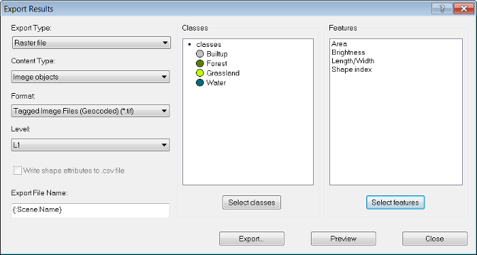
Selecting raster file from the Export Type drop-down box allows you to export image objects or classifications as raster layers together with attribute tables in csv format containing parameter values.
Image objects or classifications can be exported together with their attributes. Each image object has a unique object or class ID and the information is stored in an attached attribute table linked to the image layer. Any geo-referencing information used to create a project will be exported as well.
There are two possible locations for saving exported files:
To export image objects or classifications, open the Export Results dialog box by choosing Export > Export Results from the main menu.
To export statistics open the Export Results dialog box by choosing Export > Export Results from the main menu. (The rounding of floating point numbers depends on the operating system and runtime libraries. Therefore the results of statistical calculations between Linux and Windows may be slightly different.)
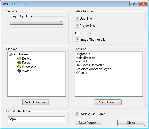
Generate Report creates a HTML page containing information about image object features and optionally a thumbnail image. To open the Generate Report dialog box, choose Export > Generate Report from the main menu.
Polygons, lines, or points of selected classes can be exported as shapefiles. As with the Export Raster File option, image objects can be exported together with their attributes and classifications. Any geo-referencing information as provided when creating a map is exported as well. The main difference to exporting image objects is that the export is not confined to polygons based on the image objects.
You can choose between three basic shape formats: points, lines and polygons. To export results as shapes, open the Export Results dialog box by choosing Export > Export Results on the main menu.
Exporting the current view is an easy way to save the map view at the current scene scale to file, which can be opened and analyzed in other applications. This export type does not include additional information such as geo-referencing, features or class assignments. To reduce the image size, you can rescale it before exporting.
1 By default, the connectors for predefined import are stored in the installation folder under \bin\drivers\import. If you want to use a different storage folder, you can change this setting under Tools > Options > General. (↑)
2 When working with a complex folder structure in a workspace, make sure that folder names are short. This is important, because project names are internally used for file names and must not be longer than 255 characters including the path, backslashes, names, and file extension. (↑)
© 2019, Trimble Inc. All rights reserved. 